机器学习中的Monte Carlo(笔记和python实现)

机器学习中的Monte-Carlo

来说一下机器学习中Monte-Carlo中用在什么地方:

  • 贝叶斯推论和学习:
    • 归一化:$p(x | y) =\frac{p(y | x)p(x)}{\int_Xp(y| x’)p(x’)dx’}$
    • 边缘概率的计算:$p(x | y) = \int_Z p(x, z | y)dz$
    • 求期望:$E_{p(x|y)}(f(x)) = \int_Xf(x)p(x|y)dx$
  • 上面三处都用到了积分,Monte-Carlo的核心思想即用样本的和去近似积分

随机采样介绍

所谓采样,实际上是指根据某种分布去生成一些数据点,比如“石头剪刀布”的游戏,服从均匀分布,且概率都是三分之一,采样即希望随机获得一个“石头”或者“剪刀”或者“布”,并且每中情况出现的机会应该是一样的。也就是说,这是我们根据观察数据再确定分布的过程的逆过程

最基本的假设是认为我们可以获得服从均匀分布的随机数。一般的采样问题,都可以理解成:有了均匀分布(简单分布)的采样,如何去获取复杂分布的采样。

离散分布采样

对于离散的分布,比如$p(x)=[0.1, 0.5, 0.2, 0.2]^T$,那么我们可以从$u \sim
U_{(0,1)}$中采样,把概率分布向量看做一个区间段,然后判断$u$落在哪个区间段内。区间段的长度和概率成正比,这样采样完全符合原来的分布。
通过一个例子实现:

假设上面的向量,分别对应“你”,“好”,“合”,“协”四个字分别出现的概率,那么我们随机采样几次,看看出现的结果。

1
2
3
4
5
6
7
8
9
10
11
12
13
14
15
16
17
18
19
20
21
import numpy as np

index2word = ["你","好","合","协"]

def sample_discrete(vec):
u = np.random.rand()
start = 0
for i, num in enumerate(vec):
if u > start:
start += num
else:
return i-1
return i

count = dict([(w, 0) for w in index2word])
# 采样1000次
for i in range(1000):
s = sample_discrete([0.1, 0.5, 0.2, 0.2])
count[index2word[s]] += 1
for k in count:
print(k," : ", count[k])
1
2
3
4
你  :  110
好 : 493
协 : 216
合 : 181

可以看到采样的频率比较符合设定的概率分布:$[0.1,0.5,0.2,0.2]$

连续分布采样

对于连续的分布,如果可以计算这个分布的累积分布函数(CDF),就可以通过计算CDF的反函数,结合基础的均匀分布,获得其采样。所以,在这个基础上我们又可以获得一些简单的分布的采样。

Box-Muller算法

Box-Muller算法,实现对高斯分布的采样。

原理:

  • 假设随机变量$x,y$都服从标准高斯分布,则有:$f(x,y) =
    \frac{1}{\sqrt{2\pi}}e^{-x^2/2}\frac{1}{\sqrt{2\pi}}e^{-y^2/2}=\frac{1}{\sqrt{2\pi}}e^{-(x^2+y^2)/2}$。
  • 如果使用极坐标系,即$x=rsin(\theta)$,$y=rcos(\theta)$,有$r^2 = x^2+y^2$。
  • 求CDF:$P(r\leq R) = \int_{r=0}^R\int_{\theta=0}^{2\pi}\frac{1}{2\pi}e^{r^2}r;drd\theta=\int_{r=0}^r=e^{-r^2}r;dr$
  • 用$s=\frac{1}{2}r^2$带入,得:$P(r\leq R) = \int _{s=0}^{r^2/2}e^{-s}ds = 1 - e^{-r^2/2}$
  • 则,随机采样$\theta$服从均与分布,范围是$0 \leq \theta \leq 1$,可以使$\theta=2\pi U_1$。
  • $1-e^{-r^2/2}=1-U_2$即$r=\sqrt{-1ln(U_2)}$

算法流程

  • 抽样两个服从均匀分布的随机数:$0
    \leq U_1, U_2, \leq 1$。
  • 令$\theta = 2\pi U_1$,$r=\sqrt{-2ln(U_2)}$
  • $x=rsin(\theta)$,$y=rcos(\theta)$ 都是服从标准高斯分布的变量。
1
2
3
4
5
6
7
8
9
10
11
12
13
14
15
16
17
18
19
20
21
22
23
24
25
26
27
28
29
30
31
32
33
34
35
36
37
38
# Code from Chapter 14 of Machine Learning: An Algorithmic Perspective
# by Stephen Marsland (http://seat.massey.ac.nz/personal/s.r.marsland/MLBook.html)

# You are free to use, change, or redistribute the code in any way you wish for
# non-commercial purposes, but please maintain the name of the original author.
# This code comes with no warranty of any kind.

# Stephen Marsland, 2008

# The Box-Muller algorithm for constructing pseudo-random Gaussian-distributed numbers

from pylab import *
import numpy as np

def boxmuller(n):

x = np.zeros((n,2))
y = np.zeros((n,2))

for i in range(n):
x[i,:] = np.array([2,2])
x2 = x[i,0]*x[i,0]+x[i,1]*x[i,1]
while (x2)>1:
x[i,:] = np.random.rand(2)*2-1
x2 = x[i,0]*x[i,0]+x[i,1]*x[i,1]

y[i,:] = x[i,:] * np.sqrt((-2*log(x2))/x2)

y = np.reshape(y,2*n,1)
return y

y = boxmuller(1000)
hist(y,normed=1,fc='c')
x = arange(-4,4,0.1)
plot(x,1/np.sqrt(2*np.pi)*np.exp(-0.5*x**2),'g',lw=6)
xlabel('x',fontsize=24)
ylabel('p(x)',fontsize=24)
show()

接下来,我们专注于复杂的任意分布的采样。

拒绝采样

拒绝采样(Rejection Sampling)。

假设我们已经可以抽样高斯分布q(x)(如Box–Muller_transform 算法),我们按照一定的方法拒绝某些样本,达到接近$p(x)$分布的目的:

reject

具体操作:

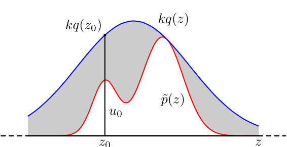
  • 首先,确定常量$k$,使得$p(x)$总在$kq(x)$的下方。
  • $x$轴方向:从$q(x)$分布抽样得到$a$。但是$a$并不一定留下,会有一定的几率被拒绝
  • $y$轴方向:从均匀分布$(0,kq(a))$中抽样得到$u$。如果$u>p(a)$,也就是落到了灰色的区域中,拒绝,否则接受这次抽样。

拒绝采样实现:

1
2
3
4
5
6
7
8
9
10
11
12
13
14
15
16
17
18
19
20
21
22
23
24
25
26
27
28
29
30
31
32
33
34
35
36
37
38
39
40
41
42
43
44
45
46
47
48
49
50
51
52
53
54
55
56
# Code from Chapter 14 of Machine Learning: An Algorithmic Perspective
# The basic rejection sampling algorithm
# 稍有修改,使用matplotlib

%matplotlib inline
import matplotlib
import numpy as np
import matplotlib.pyplot as plt
import seaborn

def qsample():
"""使用均匀分布作为q(x),返回采样"""
return np.random.rand()*4.

def p(x):
"""目标分布"""
return 0.3*np.exp(-(x-0.3)**2) + 0.7* np.exp(-(x-2.)**2/0.3)

def rejection(nsamples):

M = 0.72#0.8 k值
samples = np.zeros(nsamples,dtype=float)
count = 0
for i in range(nsamples):
accept = False
while not accept:
x = qsample()
u = np.random.rand()*M
if u<p(x):
accept = True
samples[i] = x
else:
count += 1
print "reject count: ", count
return samples

x = np.arange(0,4,0.01)
x2 = np.arange(-0.5,4.5,0.1)
realdata = 0.3*np.exp(-(x-0.3)**2) + 0.7* np.exp(-(x-2.)**2/0.3)
box = np.ones(len(x2))*0.75#0.8
box[:5] = 0
box[-5:] = 0
plt.plot(x,realdata,'g',lw=3)
plt.plot(x2,box,'r--',lw=3)

import time
t0=time.time()
samples = rejection(10000)
t1=time.time()
print "Time ",t1-t0

plt.hist(samples,15,normed=1,fc='c')
plt.xlabel('x',fontsize=24)
plt.ylabel('p(x)',fontsize=24)
plt.axis([-0.5,4.5,0,1])
plt.show()

在高维的情况下,Rejection Sampling有两个问题:

  1. 合适的q分布很难找
  2. 很难确定一个合理的k值

导致拒绝率很高。

重要性采样

重要性采样(Importance Sampling)。

$$E(f)= \int p(x)f(x) dx$$

$$ = \int q(x)\frac{p(x)f(x)}{q(x)} dx$$

其中可以把$w(x)=\frac{p(x)}{q(x)}$称为重要性权重(importance weight)

重要性采样算法

  • 从简单分布$q(x)$中采样N个样本$x^{(i)}$
  • 计算归一化的重要性权重:$w^{(i)} =\frac{p(x^{(i)})/q(x^{(i)})}{\sum_j p(x^{(j)})/q(x^{(j)})}$
  • 再在分布${x^{(i)}}$中,按照权重$w^{(i)}$作为概率做采样。
1
2
3
4
5
6
7
8
9
10
11
12
13
14
15
16
17
18
19
20
21
22
23
24
25
26
27
28
29
30
31
32
33
34
35
36
37
38
39
40
41
42
43
44
45
46
47
48
49
50
51
def qsample():
return np.random.rand()*4.

def p(x):
return 0.3*np.exp(-(x-0.3)**2) + 0.7* np.exp(-(x-2.)**2/0.3)

def q(x):
return 4.0

def importance(nsamples):

samples = np.zeros(nsamples,dtype=float)
w = np.zeros(nsamples,dtype=float)

for i in range(nsamples):
samples[i] = qsample()
w[i] = p(samples[i])/q(samples[i])

return samples, w

def sample_discrete(vec):
u = np.random.rand()
start = 0
for i, num in enumerate(vec):
if u > start:
start += num
else:
return i-1
return i

def importance_sampling(nsamples):
samples, w = importance(nsamples)
final_samples = np.zeros(nsamples,dtype=float)
w = w / w.sum()
for j in range(nsamples):
final_samples[j] = samples[sample_discrete(w)]
return final_samples

x = np.arange(0,4,0.01)
x2 = np.arange(-0.5,4.5,0.1)
realdata = 0.3*np.exp(-(x-0.3)**2) + 0.7* np.exp(-(x-2.)**2/0.3)
box = np.ones(len(x2))*0.8
box[:5] = 0
box[-5:] = 0
plt.plot(x,realdata,'g',lw=6)
plt.plot(x2,box,'r--',lw=6)

# samples,w = importance(5000)
final_samples = importance_sampling(5000)
plt.hist(final_samples,normed=1,fc='c')
plt.show()

可以明显感觉到重要性采样,速度比较慢。

MCMC

MCMC(Markov Chain Monte Carlo),上面提到的方法都是可以并行的,即某一个样本的产生不依赖于上一个样本的抽样;MCMC是一个链式的抽样过程,即每一个样本抽样跟且只跟上一个样本的抽样相关。

因此我们引入概率转移矩阵$T$,即某一时刻是状态$s$,那么下一时刻状态是$s’$的概率是:$T(s,s’)$,于是问题变转换成了某一时刻有一个抽样,那么下一个时刻抽样的概率由$T$决定。

另外,不要忘了,不管是从什么状态开始抽样,我们都期望在第$i$次的分布概率$p(x^{(i)})$可以收敛到实际分布$p(x)$。
马尔科夫链若收敛,$T$需要满足:

  • 不可化简(irreducibility):即对于x任何可能的取值,都有机会(概率大于0)到达其他的取值(不一定要下一期,只要是在有限的时刻内),即上面的图是闭环的。
  • 非周期的(aperiodicity)
  • 细致平稳条件(detail balance)$p(x)T(x,x’)=p(x’)T(x’,x)$,保证了chain是reversible。

关键:构造转移矩阵$T$,使得平稳分布恰好是我们需要的分布$p(x)$。

Metropolis-Hastings Algorithm

Metropolis-Hastings的核心思想类似于拒绝采样:我们有一个采样$x^*$,要决定是否留下它。类似的,我们也有一个建议分布$q(x_i|x_{i-1})$。和拒绝采样不同的是,一旦拒绝新的采样,将采样当前的采样作为新采样。这也是这个算法之所以高效的原因。

算法介绍:对于目标分布$p(x)$,首先给定参考条件概率分布$q(x^*|x)$,然后基于当前x的抽样一个新样本$x^*$,然后依据一定的概率移动到$x^*$(否则还留在$x$),这个概率是接受概率$A(x_i,x^*)=min{1,\frac{p(x^*)q(x_i|x^*)}{p(x_i)q(x^*|x_i)}}$

接受概率的推导:上面的细致平稳条件:$p(x)T(x,x’)=p(x’)T(x’,x)$,我们希望根据一个建议分布$q$和一个接受率$a$来等价于$T$。即:$p(i)q(i,j)a(i, j) = p(j)q(j,i)a(j,i)$。令$a(j,i)=1$,有$a(i,j)=\frac{p(j)q(j,i)}{p(i)q(j,i)}$。注:这段推导的符号标记和全文的风格不太相同,也比较简洁。

算法流程

  • 给顶一个初始值$x_0$
  • 重复以下步骤:
    • 从$q(x_i|x_{i-1})$中采样一个样本$x^*$。
    • 从均匀分布中抽样一个$u$。
    • 如果$u<A(x_i,x^*)$
      • $x_{i+1} = x^*$
    • 否则:
      • $x_{i+1} = x_i$

接受概率$A(x_i,x^*)$有个形象的比喻:假设你目前在一片高低不平的山地上,你此行的目的是在海拔越高的地方停留越久($p(x)$大的时候,样本里$x$就多)。你的方法是随便指一个新的地方,如果这个地方的海拔更高,那么就移动过去;但如果这个地方的海拔比当前低,你就抛一个不均匀的硬币决定是否过去,而硬币的不均匀程度相当于新海拔和当前海拔的比例。也即新海拔若是当前海拔的一半,你就只有1/2的概率会过去。MH算法中$q(x^*|x_i)$就是按照一定的规律指出一个新方向,$A(x_i,x^*)$就是计算相对高度。

基于上述想法的MH算法实现:

1
2
3
4
5
6
7
8
9
10
11
12
13
14
15
16
17
18
19
20
21
22
23
24
25
26
27
28
29
30
31
# my own try 
import scipy.stats
mu = 3
sigma = 10
def qsample():
return np.random.normal(mu,sigma)
def q(x):
return exp(-(x-mu)**2/(sigma**2))
def p(x):
"""目标分布"""
return 0.3*np.exp(-(x-0.3)**2) + 0.7* np.exp(-(x-2.)**2/0.3)
def hm(n=10000):
sample = np.zeros(n)
sample[0] = 0.5
for i in range(n-1):
q_s = qsample()
u = np.random.rand()
if u < min(1, (p(q_s)*q(sample[i]))/(p(sample[i])*q(q_s))):
sample[i+1] = q_s
else:
sample[i+1] = sample[i]
return sample

x = np.arange(0,4,0.1)
realdata = p(x)
N=10000
sample = hm(N)
plt.plot(x,realdata,'g',lw=3)
plt.plot(x,q(x),'r')
plt.hist(sample,bins=x,normed=1,fc='c')
plt.show()

1
2
3
4
5
6
7
8
9
10
11
12
13
14
15
16
17
18
19
20
21
22
23
24
25
26
27
28
29
30
31
32
33
34
35
36
37
38
39
40
41
42
43
44
45
46
47
48
49
50
51
52
53
54
55
56
57
58
59
60
61
62
63
64
65
66
67
68
69
70
71
# Code from Chapter 14 of Machine Learning: An Algorithmic Perspective
# by Stephen Marsland (http://seat.massey.ac.nz/personal/s.r.marsland/MLBook.html)

# You are free to use, change, or redistribute the code in any way you wish for
# non-commercial purposes, but please maintain the name of the original author.
# This code comes with no warranty of any kind.

# Stephen Marsland, 2008

# The Metropolis-Hastings algorithm
from pylab import *
from numpy import *

def p(x):
mu1 = 3
mu2 = 10
v1 = 10
v2 = 3
return 0.3*exp(-(x-mu1)**2/v1) + 0.7* exp(-(x-mu2)**2/v2)

def q(x):
mu = 5
sigma = 10
return exp(-(x-mu)**2/(sigma**2))

stepsize = 0.5
x = arange(-10,20,stepsize)
px = zeros(shape(x))
for i in range(len(x)):
px[i] = p(x[i])
N = 5000

# independence chain
u = random.rand(N)
mu = 5
sigma = 10
y = zeros(N)
y[0] = random.normal(mu,sigma)
for i in range(N-1):
ynew = random.normal(mu,sigma)
alpha = min(1,p(ynew)*q(y[i])/(p(y[i])*q(ynew)))
if u[i] < alpha:
y[i+1] = ynew
else:
y[i+1] = y[i]

# random walk chain
u2 = random.rand(N)
sigma = 10
y2 = zeros(N)
y2[0] = random.normal(0,sigma)
for i in range(N-1):
y2new = y2[i] + random.normal(0,sigma)
alpha = min(1,p(y2new)/p(y2[i]))
if u2[i] < alpha:
y2[i+1] = y2new
else:
y2[i+1] = y2[i]

figure(1)
nbins = 30
hist(y, bins = x)
plot(x, px*N/sum(px), color='g', linewidth=2)
plot(x, q(x)*N/sum(px), color='r', linewidth=2)

figure(2)
nbins = 30
hist(y2, bins = x)
plot(x, px*N/sum(px), color='g', linewidth=2)

show()

Gibbs Sampling

Gibbs Sampling的本质是MH的变种。适用于我们知道完全条件概率的情况,即$p(x_j|x_1,…,x_{j-1},x_{j+1},…,x_n)$,也写作:$p(x_j|x_{-j})$。

采用设置多维概率分布$p$里的完全条件概率(full conditionals)作为建议概率(proposal),q,那么接受率就会始终=1,一直接受$x^*$。

对 $j=1,…,n$

注意符号的问题,在MH算法中,$x_i$代表第i个样本的值,在Gibbs中,$x_j^{(i)}$代表第i个样本中,第j维(第j个变量)的值。

证明:
$$A(x^{(i)},x^*)=min\{1,\frac{p(x^*)q(x^{(i)}|x^*)}{p(x^{(i)})q(x^*|x^{(i)})}\}$$

$$=min\{1,\frac{p(x^*)p(x^{(i)}_j|x^{(i)}_{-j})}{p(x^{(i)})p(x^*_j|x^*_{-j})}\}$$

$$=min\{1,\frac{p(x^*_{-j})}{p(x^{(i)}_{-j})}\}$$

$$=1$$

Gibbs Sampling算法

  • 对每个变量$x_j$:
    • 初始化$x_j^{(0)}$
  • 重复:
    • 对每个变量$x_j$:
  • 从$p(x_1 | x_{2}^{(i)}, … , x_{n}^{(i)})$中采样$x_1^{i+1}$。
    • 从$p(x_2 | x_{1}^{(i+1)}, x_{3}^{(i)}, …, x_{n}^{(i)})$中采样$x_2^{i+1}$。
    • 从$p(x_n | x_{1}^{(i+1)}, …, x_{n-1}^{(i+1)})$中采样$x_n^{i+1}$。
  • 直到有足够多的sample。
1
2
3
4
5
6
7
8
9
10
11
12
13
14
15
16
17
18
19
20
21
22
23
24
25
26
27
28
29
30
31
32
33
34
35
36
37
38
39
40
41
42
43
# Code from Chapter 14 of Machine Learning: An Algorithmic Perspective
# A simple Gibbs sampler

def pXgivenY(y,m1,m2,s1,s2):
return np.random.normal(m1 + (y-m2)/s2,s1)

def pYgivenX(x,m1,m2,s1,s2):
return np.random.normal(m2 + (x-m1)/s1,s2)

def gibbs(N=5000):
k=20
x0 = np.zeros(N,dtype=float)
m1 = 10
m2 = 20
s1 = 2
s2 = 3
for i in range(N):
y = np.random.rand(1)
# 每次采样需要迭代 k 次
for j in range(k):
x = pXgivenY(y,m1,m2,s1,s2)
y = pYgivenX(x,m1,m2,s1,s2)
x0[i] = x

return x0

def f(x):
"""目标分布"""
return np.exp(-(x-10)**2/10)

# 画图
N=10000
s=gibbs(N)
x1 = np.arange(0,17,1)
plt.hist(s,bins=x1,fc='c')
x1 = np.ar
ange(0,17, 0.1)
px1 = np.zeros(len(x1))
for i in range(len(x1)):
px1[i] = f(x1[i])
plt.plot(x1, px1*N*10/sum(px1), color='r',linewidth=3)

plt.show()

以上算法是简单的二维Gibbs Sampling的实现,如下图:
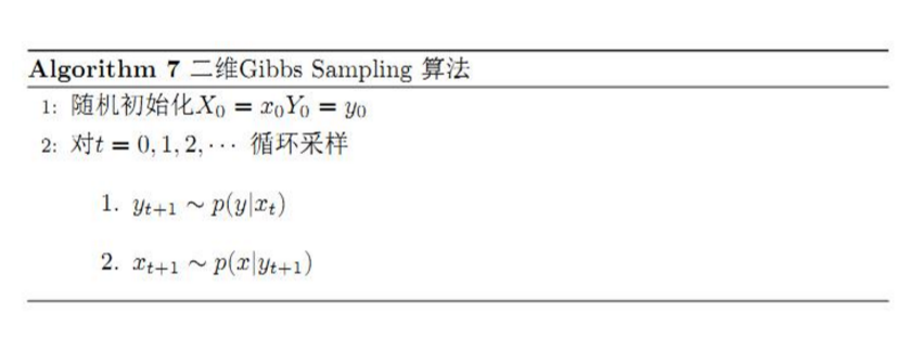
参考资料: